Types
Regression
- A supervised problem, the outputs are continuous rather than discrete.
Classification
- Inputs are divided into two or more classes, and the learner must produce a model that assigns unseen inputs to one or more (multi-label classification) of these classes. This is typically tackled in a supervised way.
Clustering
- A set of inputs is to be divided into groups. Unlike in classification, the groups are not known beforehand, making this typically an unsupervised task.
Density Estimation
- Finds the distribution of inputs in some space.
Dimensionality Reduction
- Simplifies inputs by mapping them into a lower-dimensional space.
Kind
Parametric
Step 1: Making an assumption about the functional form or shape of our function (f), i.e.: f is linear, thus we will select a linear model.
Step 2: Selecting a procedure to fit or train our model. This means estimating the Beta parameters in the linear function. A common approach is the (ordinary) least squares, amongst others.
Non-Parametric
- When we do not make assumptions about the form of our function (f). However, since these methods do not reduce the problem of estimating f to a small number of parameters, a large number of observations is required in order to obtain an accurate estimate for f. An example would be the thin-plate spline model.
Categories
Supervised
- The computer is presented with example inputs and their desired outputs, given by a "teacher", and the goal is to learn a general rule that maps inputs to outputs.
Unsupervised
- No labels are given to the learning algorithm, leaving it on its own to find structure in its input. Unsupervised learning can be a goal in itself (discovering hidden patterns in data) or a means towards an end (feature learning).
Reinforcement Learning
- A computer program interacts with a dynamic environment in which it must perform a certain goal (such as driving a vehicle or playing a game against an opponent). The program is provided feedback in terms of rewards and punishments as it navigates its problem space.
Approaches
Decision tree learning
Association rule learning
Artificial neural networks
Deep learning
Inductive logic programming
Support vector machines
Clustering
Bayesian networks
Reinforcement learning
Representation learning
Similarity and metric learning
Sparse dictionary learning
Genetic algorithms
Rule-based machine learning
Learning classifier systems
Taxonomy
Generative Methods
Popular models
Mixtures of Gaussians, Mixtures of experts, Hidden Markov Models (HMM)
Gaussians, Naïve Bayes, Mixtures of multinomials
Sigmoidal belief networks, Bayesian networks, Markov random fields
Model class-conditional pdfs and prior probabilities. “Generative” since sampling can generate synthetic data points.
Discriminative Methods
Directly estimate posterior probabilities. No attempt to model underlying probability distributions. Focus computational resources on given task– better performance
Popular Models
Logistic regression, SVMs
Traditional neural networks, Nearest neighbor
Conditional Random Fields (CRF)
Selection Criteria
Prediction Accuracy vs Model Interpretability
- There is an inherent tradeoff between Prediction Accuracy and Model Interpretability, that is to say that as the model get more flexible in the way the function (f) is selected, they get obscured, and are hard to interpret. Flexible methods are better for inference, and inflexible methods are preferable for prediction.
Libraries
Python
Numpy
- Adds support for large, multi-dimensional arrays and matrices, along with a large library of high-level mathematical functions to operate on these arrays
Pandas
- Offers data structures and operations for manipulating numerical tables and time series
Scikit-Learn
- It features various classification, regression and clustering algorithms including support vector machines, random forests, gradient boosting, k-means and DBSCAN, and is designed to interoperate with the Python numerical and scientific libraries NumPy and SciPy.
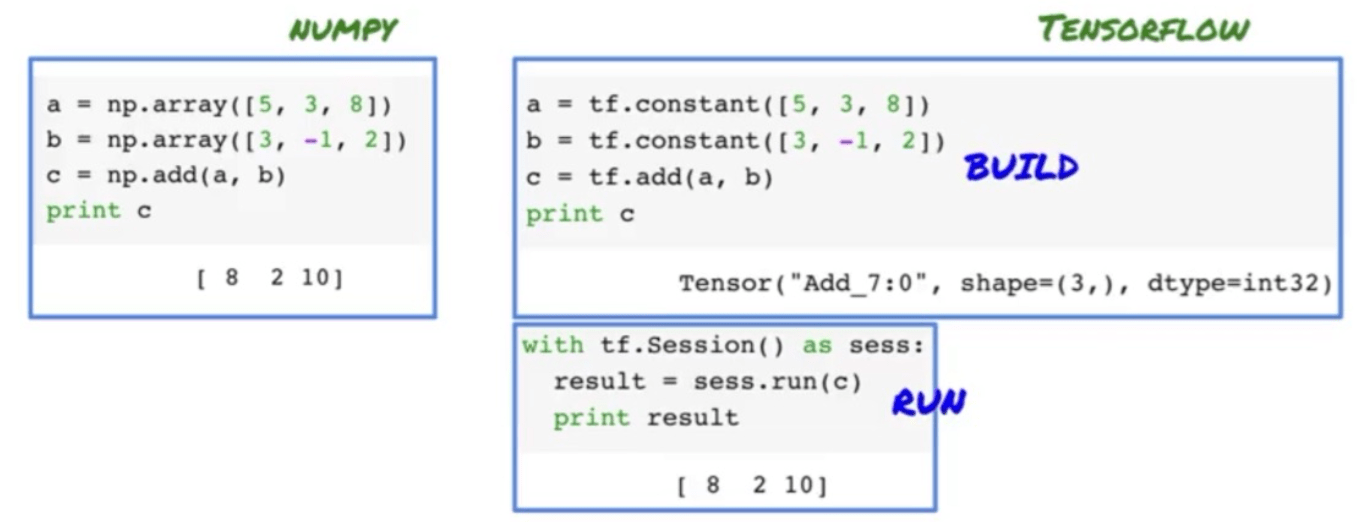
Tensorflow
Components
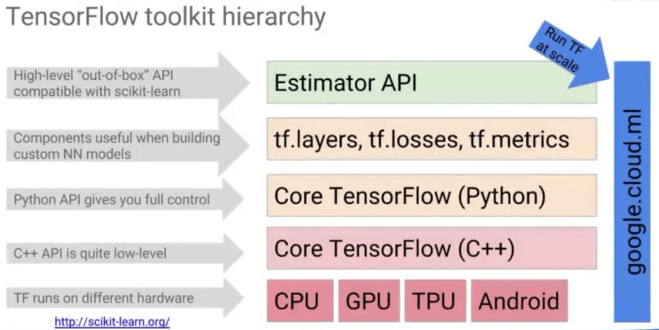
Does lazy evaluation. Need to build the graph, and then run it in a session.
MXNet
- Is an modern open-source deep learning framework used to train, and deploy deep neural networks. MXNet library is portable and can scale to multiple GPUs and multiple machines. MXNet is supported by major Public Cloud providers including AWS and Azure. Amazon has chosen MXNet as its deep learning framework of choice at AWS.
Keras
- Is an open source neural network library written in Python. It is capable of running on top of MXNet, Deeplearning4j, Tensorflow, CNTK or Theano. Designed to enable fast experimentation with deep neural networks, it focuses on being minimal, modular and extensible.
Torch
- Torch is an open source machine learning library, a scientific computing framework, and a script language based on the Lua programming language. It provides a wide range of algorithms for deep machine learning, and uses the scripting language LuaJIT, and an underlying C implementation.
Microsoft Cognitive Toolkit
- Previously known as CNTK and sometimes styled as The Microsoft Cognitive Toolkit, is a deep learning framework developed by Microsoft Research. Microsoft Cognitive Toolkit describes neural networks as a series of computational steps via a directed graph.
Tuning
Cross-validation
One round of cross-validation involves partitioning a sample of data into complementary subsets, performing the analysis on one subset (called the training set), and validating the analysis on the other subset (called the validation set or testing set). To reduce variability, multiple rounds of cross-validation are performed using different partitions, and the validation results are averaged over the rounds.
Methods
Leave-p-out cross-validation
Leave-one-out cross-validation
k-fold cross-validation
Holdout method
Repeated random sub-sampling validation

Hyperparameters
Grid Search
- The traditional way of performing hyperparameter optimization has been grid search, or a parameter sweep, which is simply an exhaustive searching through a manually specified subset of the hyperparameter space of a learning algorithm. A grid search algorithm must be guided by some performance metric, typically measured by cross-validation on the training set or evaluation on a held-out validation set.
Random Search
- Since grid searching is an exhaustive and therefore potentially expensive method, several alternatives have been proposed. In particular, a randomized search that simply samples parameter settings a fixed number of times has been found to be more effective in high-dimensional spaces than exhaustive search.
Gradient-based optimization
- For specific learning algorithms, it is possible to compute the gradient with respect to hyperparameters and then optimize the hyperparameters using gradient descent. The first usage of these techniques was focused on neural networks. Since then, these methods have been extended to other models such as support vector machines or logistic regression.
Early Stopping (Regularization)
- Early stopping rules provide guidance as to how many iterations can be run before the learner begins to over-fit, and stop the algorithm then.
Overfitting
- When a given method yields a small training MSE (or cost), but a large test MSE (or cost), we are said to be overfitting the data. This happens because our statistical learning procedure is trying too hard to find pattens in the data, that might be due to random chance, rather than a property of our function. In other words, the algorithms may be learning the training data too well. If model overfits, try removing some features, decreasing degrees of freedom, or adding more data.
Underfitting
- Opposite of Overfitting. Underfitting occurs when a statistical model or machine learning algorithm cannot capture the underlying trend of the data. It occurs when the model or algorithm does not fit the data enough. Underfitting occurs if the model or algorithm shows low variance but high bias (to contrast the opposite, overfitting from high variance and low bias). It is often a result of an excessively simple model.
Bootstrap
- Test that applies Random Sampling with Replacement of the available data, and assigns measures of accuracy (bias, variance, etc.) to sample estimates.
Bagging
- An approach to ensemble learning that is based on bootstrapping. Shortly, given a training set, we produce multiple different training sets (called bootstrap samples), by sampling with replacement from the original dataset. Then, for each bootstrap sample, we build a model. The results in an ensemble of models, where each model votes with the equal weight. Typically, the goal of this procedure is to reduce the variance of the model of interest (e.g. decision trees).
Performance Analysis
Confusion Matrix
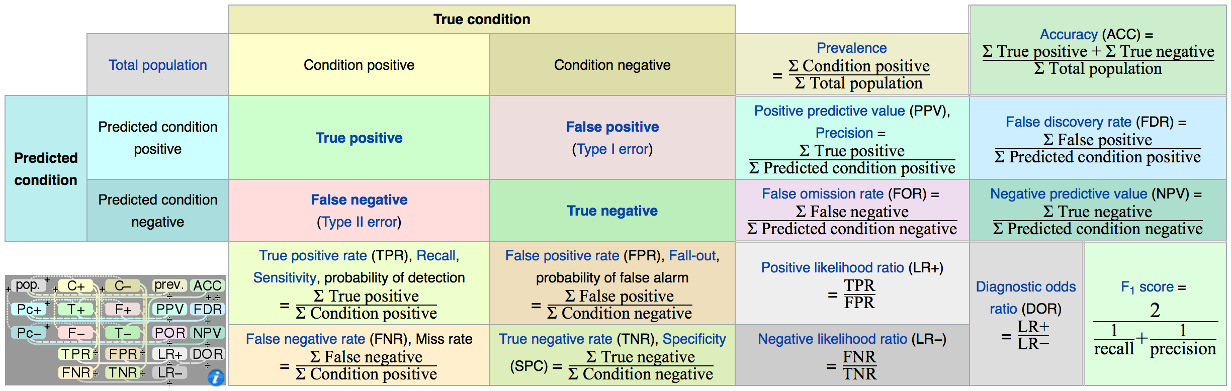
Accuracy
- Fraction of correct predictions, not reliable as skewed when the data set is unbalanced (that is, when the number of samples in different classes vary greatly)
f1 score
Precision
- Out of all the examples the classifier labeled as positive, what fraction were correct?
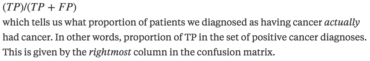
- Out of all the examples the classifier labeled as positive, what fraction were correct?
Recall
- Out of all the positive examples there were, what fraction did the classifier pick up?
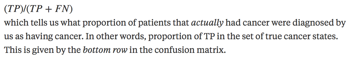
- Out of all the positive examples there were, what fraction did the classifier pick up?
Harmonic Mean of Precision and Recall: (2 * p * r / (p + r))
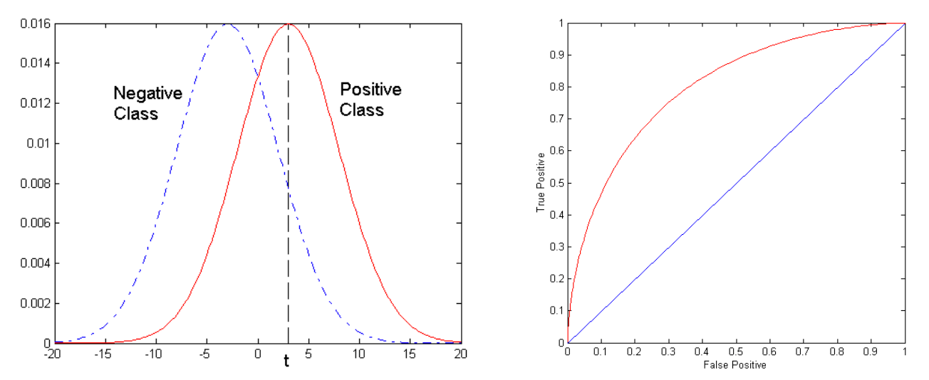
ROC Curve - Receiver Operating Characteristics
- True Positive Rate (Recall / Sensitivity) vs False Positive Rate (1-Specificity)
Bias-Variance Tradeoff
Bias refers to the amount of error that is introduced by approximating a real-life problem, which may be extremely complicated, by a simple model. If Bias is high, and/or if the algorithm performs poorly even on your training data, try adding more features, or a more flexible model.
Variance is the amount our model’s prediction would change when using a different training data set. High: Remove features, or obtain more data.
Goodness of Fit = R^2
- 1.0 - sum_of_squared_errors / total_sum_of_squares(y)
Mean Squared Error (MSE)
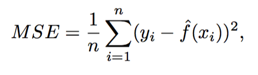
- The mean squared error (MSE) or mean squared deviation (MSD) of an estimator (of a procedure for estimating an unobserved quantity) measures the average of the squares of the errors or deviations—that is, the difference between the estimator and what is estimated.
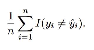
Error Rate
The proportion of mistakes made if we apply out estimate model function the the training observations in a classification setting.
Motivation
Prediction
- When we are interested mainly in the predicted variable as a result of the inputs, but not on the each way of the inputs affect the prediction. In a real estate example, Prediction would answer the question of: Is my house over or under valued? Non-linear models are very good at these sort of predictions, but not great for inference because the models are much less interpretable.
Inference
- When we are interested in the way each one of the inputs affect the prediction. In a real estate example, Inference would answer the question of: How much would my house cost if it had a view of the sea? Linear models are more suited for inference because the models themselves are easier to understand than their non-linear counterparts.
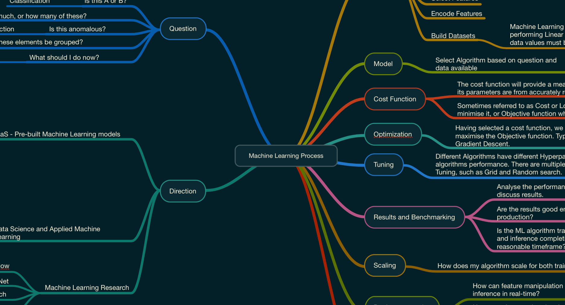
Machine Learning Process
Data
Find
Collect
Explore
Clean Features
Impute Features
Engineer Features
Select Features
Encode Features
Build Datasets
- Machine Learning is math. In specific, performing Linear Algebra on Matrices. Our data values must be numeric.
Model
Select Algorithm based on question and data available
Cost Function
The cost function will provide a measure of how far my algorithm and its parameters are from accurately representing my training data.
Sometimes referred to as Cost or Loss function when the goal is to minimise it, or Objective function when the goal is to maximise it.
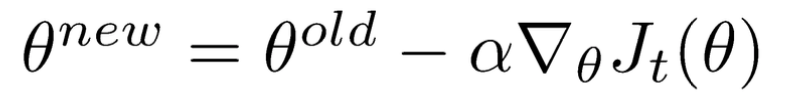
Optimization
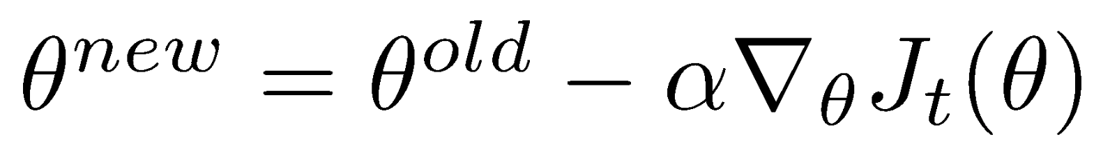
Having selected a cost function, we need a method to minimise the Cost function, or maximise the Objective function. Typically this is done by Gradient Descent or Stochastic Gradient Descent.
Tuning
Different Algorithms have different Hyperparameters, which will affect the algorithms performance. There are multiple methods for Hyperparameter Tuning, such as Grid and Random search.
Results and Benchmarking
Analyse the performance of each algorithms and discuss results.
Are the results good enough for production?
Is the ML algorithm training and inference completing in a reasonable timeframe?
Scaling
How does my algorithm scale for both training and inference?
Deployment and Operationalisation
How can feature manipulation be done for training and inference in real-time?
How to make sure that the algorithm is retrained periodically and deployed into production?
How will the ML algorithms be integrated with other systems?
Infrastructure
Can the infrastructure running the machine learning process scale?
How is access to the ML algorithm provided? REST API? SDK?
Is the infrastructure appropriate for the algorithm we are running? CPU's or GPU's?
Direction
SaaS - Pre-built Machine Learning models
Google Cloud
Vision API
Speech API
Jobs API
Video Intelligence API
Language API
Translation API
AWS
Rekognition
Lex
Polly
… many others
Data Science and Applied Machine Learning
Google Cloud
- ML Engine
AWS
- Amazon Machine Learning
Tools: Jupiter / Datalab / Zeppelin
… many others
Machine Learning Research
Tensorflow
MXNet
Torch
… many others
Question
Is this A or B?
- Classification
How much, or how many of these?
- Regression
Is this anomalous?
- Anomaly Detection
How can these elements be grouped?
- Clustering
What should I do now?
- Reinforcement Learning
Machine Learning Mathematics
Cost/Loss(Min) Objective(Max) Functions
Intuition
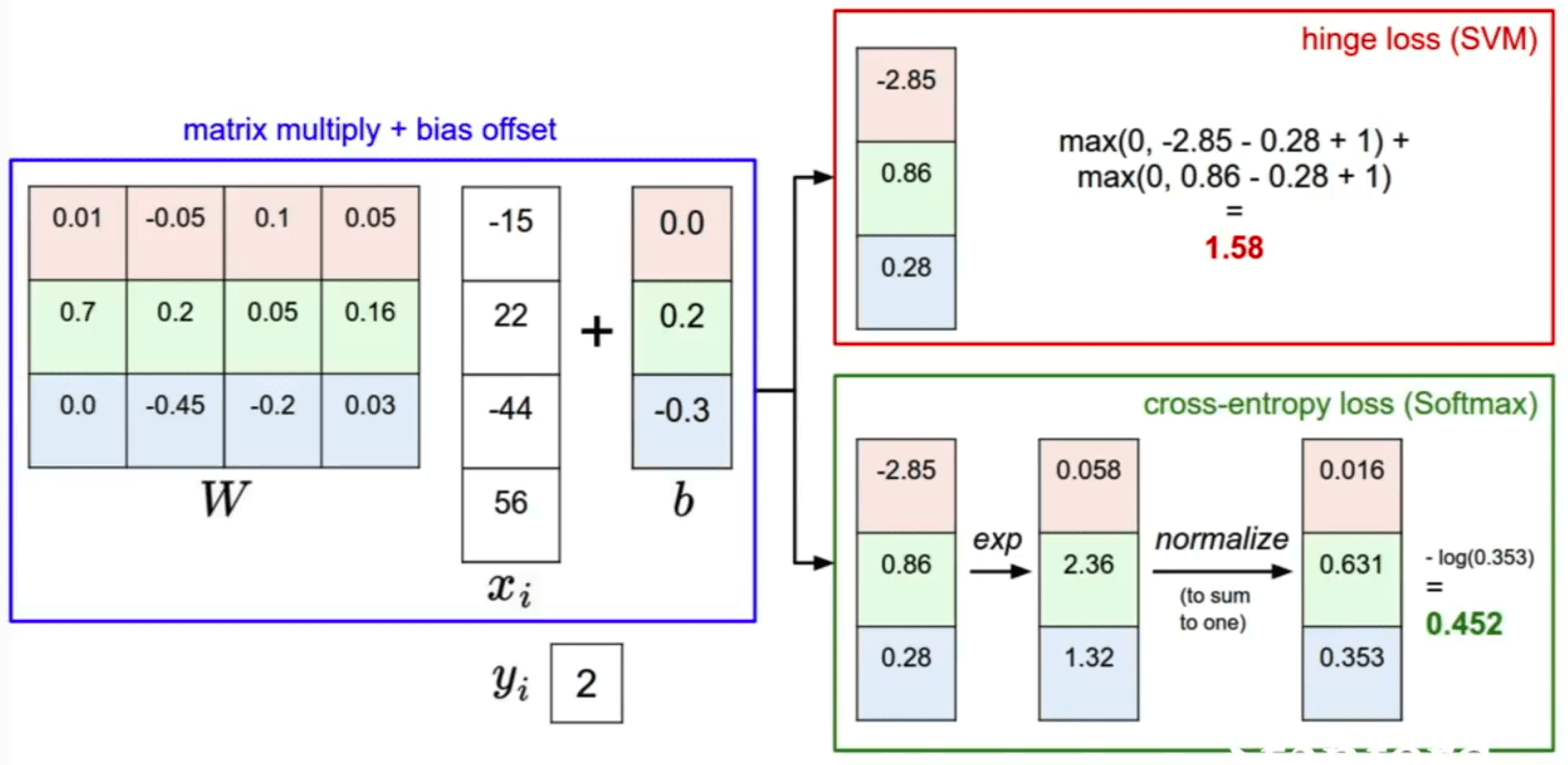
The cost function will tell us how right the predictions of our model and weight matrix are, and the choice of cost function will drive how much we care about how wrong each prediction is. For instance, a hinge loss will assume the difference between each incorrect prediction value is linear. Were we to square the hinge loss and use that as our cost function, we would be telling the system that being very wrong gets exponentially worse as we get away from the right prediction. Cross Entropy would offer a probabilistic approach.
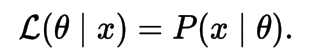
Maximum Likelihood Estimation (MLE)
Many cost functions are the result of applying Maximum Likelihood. For instance, the Least Squares cost function can be obtained via Maximum Likelihood. Cross-Entropy is another example.
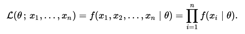
The likelihood of a parameter value (or vector of parameter values), θ, given outcomes x, is equal to the probability (density) assumed for those observed outcomes given those parameter values, that is
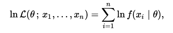
The natural logarithm of the likelihood function, called the log-likelihood, is more convenient to work with. Because the logarithm is a monotonically increasing function, the logarithm of a function achieves its maximum value at the same points as the function itself, and hence the log-likelihood can be used in place of the likelihood in maximum likelihood estimation and related techniques.
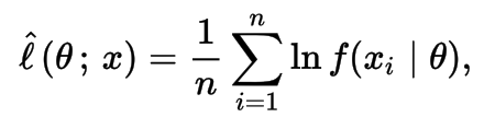
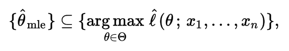
In general, for a fixed set of data and underlying statistical model, the method of maximum likelihood selects the set of values of the model parameters that maximizes the likelihood function. Intuitively, this maximizes the "agreement" of the selected model with the observed data, and for discrete random variables it indeed maximizes the probability of the observed data under the resulting distribution. Maximum-likelihood estimation gives a unified approach to estimation, which is well-defined in the case of the normal distribution and many other problems.

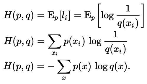
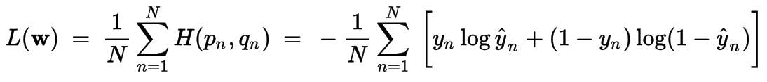
Cross-Entropy
Cross entropy can be used to define the loss function in machine learning and optimization. The true probability pi is the true label, and the given distribution qi is the predicted value of the current model.
Cross-entropy error function and logistic regression
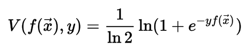
Logistic
The logistic loss function is defined as:
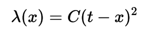
Quadratic
The use of a quadratic loss function is common, for example when using least squares techniques. It is often more mathematically tractable than other loss functions because of the properties of variances, as well as being symmetric: an error above the target causes the same loss as the same magnitude of error below the target. If the target is t, then a quadratic loss function is:
0-1 Loss
In statistics and decision theory, a frequently used loss function is the 0-1 loss function

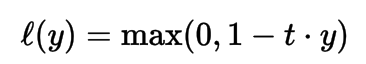
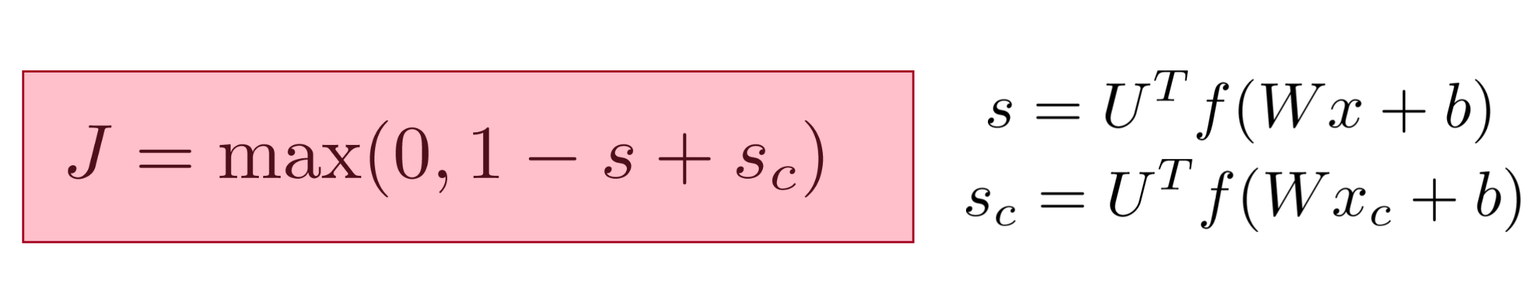
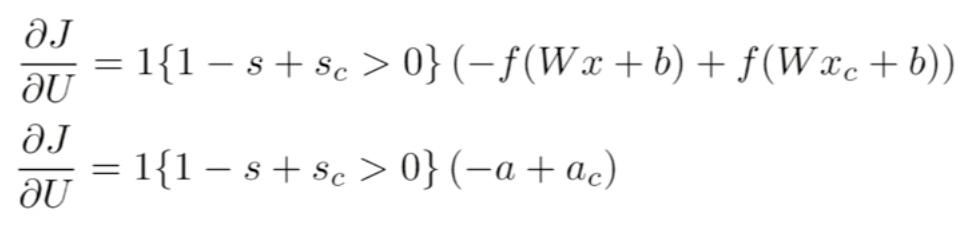
Hinge Loss
The hinge loss is a loss function used for training classifiers. For an intended output t = ±1 and a classifier score y, the hinge loss of the prediction y is defined as:
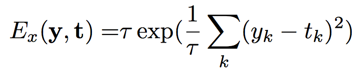
Exponential
Hellinger Distance
It is used to quantify the similarity between two probability distributions. It is a type of f-divergence.
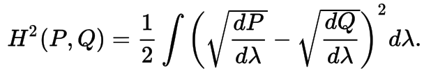
To define the Hellinger distance in terms of measure theory, let P and Q denote two probability measures that are absolutely continuous with respect to a third probability measure λ. The square of the Hellinger distance between P and Q is defined as the quantity
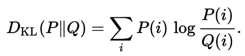
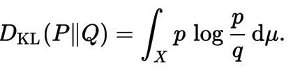
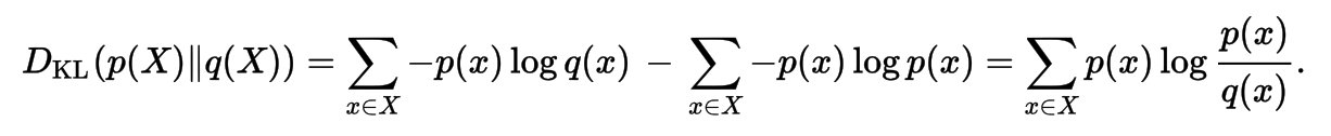
Kullback-Leibler Divengence
Is a measure of how one probability distribution diverges from a second expected probability distribution. Applications include characterizing the relative (Shannon) entropy in information systems, randomness in continuous time-series, and information gain when comparing statistical models of inference.
Discrete
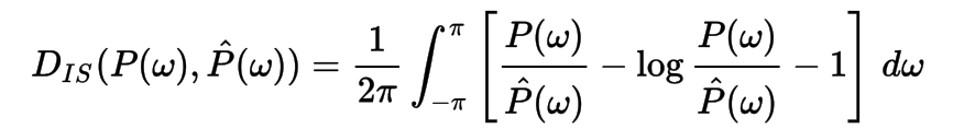
Itakura–Saito distance
is a measure of the difference between an original spectrum P(ω) and an approximation
P^(ω) of that spectrum. Although it is not a perceptual measure, it is intended to reflect perceptual (dis)similarity.
https://stats.stackexchange.com/questions/154879/a-list-of-cost-functions-used-in-neural-networks-alongside-applications
https://en.wikipedia.org/wiki/Loss_functions_for_classification
Probability
Concepts
Frequentist vs Bayesian Probability
Frequentist
- Basic notion of probability: # Results / # Attempts
Bayesian
- The probability is not a number, but a distribution itself.
http://www.behind-the-enemy-lines.com/2008/01/are-you-bayesian-or-frequentist-or.html
Random Variable
In probability and statistics, a random variable, random quantity, aleatory variable or stochastic variable is a variable whose value is subject to variations due to chance (i.e. randomness, in a mathematical sense). A random variable can take on a set of possible different values (similarly to other mathematical variables), each with an associated probability, in contrast to other mathematical variables.
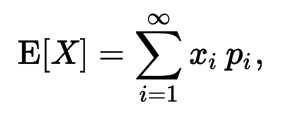
Expectation (Expected Value) of a Random Variable
- Same, for continuous variables
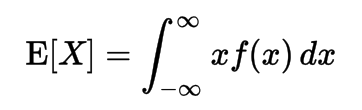
- Same, for continuous variables
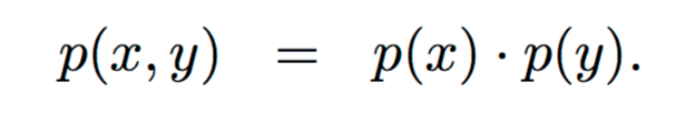
Independence
Two events are independent, statistically independent, or stochastically independent if the occurrence of one does not affect the probability of the other.
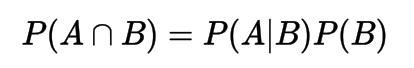
Conditionality
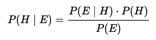
Bayes Theorem (rule, law)
Simple Form
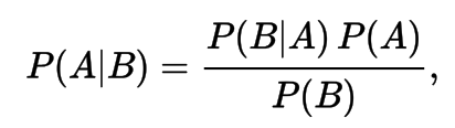
- With Law of Total probability
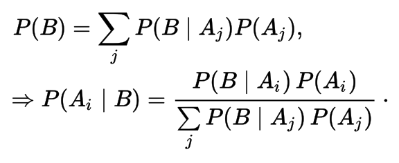
- With Law of Total probability
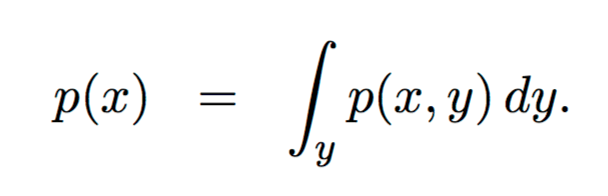
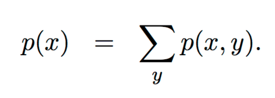
Marginalisation
The marginal distribution of a subset of a collection of random variables is the probability distribution of the variables contained in the subset. It gives the probabilities of various values of the variables in the subset without reference to the values of the other variables.
Continuous
Discrete
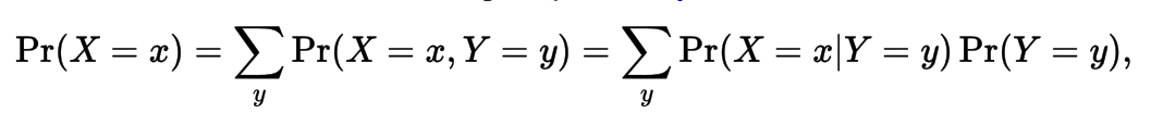
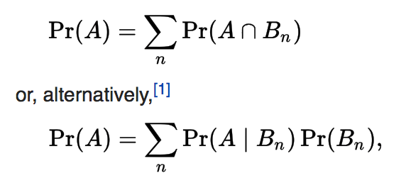
Law of Total Probability
Is a fundamental rule relating marginal probabilities to conditional probabilities. It expresses the total probability of an outcome which can be realized via several distinct events - hence the name.
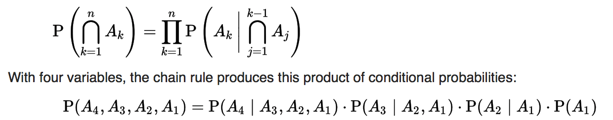
Chain Rule
- Permits the calculation of any member of the joint distribution of a set of random variables using only conditional probabilities.
- Permits the calculation of any member of the joint distribution of a set of random variables using only conditional probabilities.
Bayesian Inference
- Bayesian inference derives the posterior probability as a consequence of two antecedents, a prior probability and a "likelihood function" derived from a statistical model for the observed data. Bayesian inference computes the posterior probability according to Bayes' theorem. It can be applied iteratively so to update the confidence on out hypothesis.
- Bayesian inference derives the posterior probability as a consequence of two antecedents, a prior probability and a "likelihood function" derived from a statistical model for the observed data. Bayesian inference computes the posterior probability according to Bayes' theorem. It can be applied iteratively so to update the confidence on out hypothesis.
Distributions
Definition
- Is a table or an equation that links each outcome of a statistical experiment with the probability of occurence. When Continuous, is is described by the Probability Density Function
Types (Density Function)
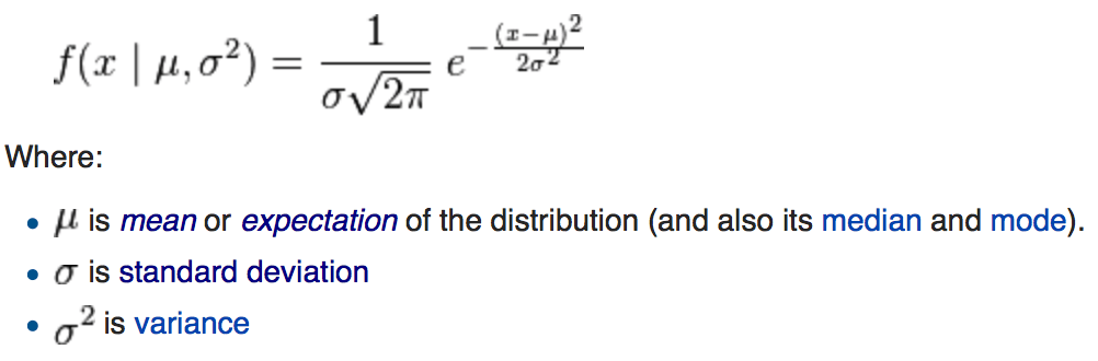
Normal (Gaussian)
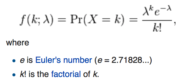
Poisson
- Uniform
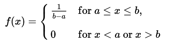
- Uniform
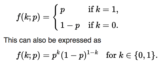
Bernoulli
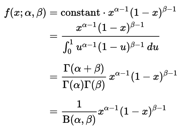
Gamma
- Binomial
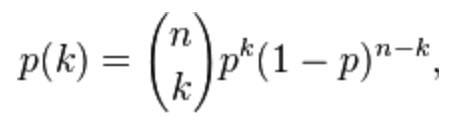
- Binomial
Cumulative Distribution Function (CDF)
Information Theory
Entropy
Entropy is a measure of unpredictability of information content.
- To evaluate a language model, we should measure how much surprise it gives us for real sequences in that language. For each real word encountered, the language model will give a probability p. And we use -log(p) to quantify the surprise. And we average the total surprise over a long enough sequence. So, in case of a 1000-letter sequence with 500 A and 500 B, the surprise given by the 1/3-2/3 model will be:
[-500log(1/3) - 500log(2/3)]/1000 = 1/2 * Log(9/2)
While the correct 1/2-1/2 model will give:
[-500log(1/2) - 500log(1/2)]/1000 = 1/2 * Log(8/2)
So, we can see, the 1/3, 2/3 model gives more surprise, which indicates it is worse than the correct model.
Only when the sequence is long enough, the average effect will mimic the expectation over the 1/2-1/2 distribution. If the sequence is short, it won't give a convincing result.
- To evaluate a language model, we should measure how much surprise it gives us for real sequences in that language. For each real word encountered, the language model will give a probability p. And we use -log(p) to quantify the surprise. And we average the total surprise over a long enough sequence. So, in case of a 1000-letter sequence with 500 A and 500 B, the surprise given by the 1/3-2/3 model will be:
Cross Entropy
- Cross entropy between two probability distributions p and q over the same underlying set of events measures the average number of bits needed to identify an event drawn from the set, if a coding scheme is used that is optimized for an "unnatural" probability distribution q, rather than the "true" distribution p.
Joint Entropy
Conditional Entropy

Mutual Information
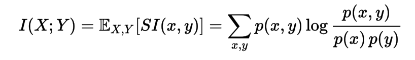
Kullback-Leibler Divergence
Density Estimation
Mostly Non-Parametric. Parametric makes assumptions on my data/random-variables, for instance, that they are normally distributed. Non-parametric does not.
The methods are generally intended for description rather than formal inference
Methods
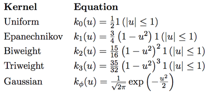
Kernel Density Estimation
non-negative
it’s a type of PDF that it is symmetric
real-valued
symmetric
integral over function is equal to 1
non-parametric
calculates kernel distributions for every sample point, and then adds all the distributions
Uniform, Triangle, Quartic, Triweight, Gaussian, Cosine, others...
Cubic Spline
- A cubic spline is a function created from cubic polynomials on each between-knot interval by pasting them together twice continuously differentiable at the knots.
Regularization
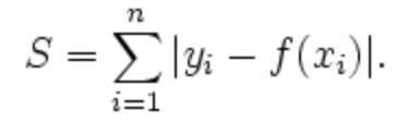
L1 norm
Manhattan Distance
L1-norm is also known as least absolute deviations (LAD), least absolute errors (LAE). It is basically minimizing the sum of the absolute differences (S) between the target value and the estimated values.
Intuitively, the L1 norm prefers a weight matrix which contains the larger number of zeros.
L2 norm
Euclidean Distance
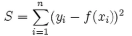
L2-norm is also known as least squares. It is basically minimizing the sum of the square of the differences (S) between the target value and the estimated values:
Intuitively, the L2 norm prefers a weight matrix where the norm is distributed across all weight matrix entries.
Early Stopping
- Early stopping rules provide guidance as to how many iterations can be run before the learner begins to over-fit, and stop the algorithm then.
Dropout
- Is a regularization technique for reducing overfitting in neural networks by preventing complex co-adaptations on training data. It is a very efficient way of performing model averaging with neural networks. The term "dropout" refers to dropping out units (both hidden and visible) in a neural network
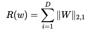
Sparse regularizer on columns
This regularizer defines an L2 norm on each column and an L1 norm over all columns. It can be solved by proximal methods.
Nuclear norm regularization

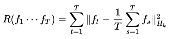
Mean-constrained regularization
This regularizer constrains the functions learned for each task to be similar to the overall average of the functions across all tasks. This is useful for expressing prior information that each task is expected to share similarities with each other task. An example is predicting blood iron levels measured at different times of the day, where each task represents a different person.
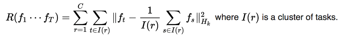
Clustered mean-constrained regularization
This regularizer is similar to the mean-constrained regularizer, but instead enforces similarity between tasks within the same cluster. This can capture more complex prior information. This technique has been used to predict Netflix recommendations.
Graph-based similarity
More general than above, similarity between tasks can be defined by a function. The regularizer encourages the model to learn similar functions for similar tasks.

Optimization
Gradient Descent
- Is a first-order iterative optimization algorithm for finding the minimum of a function. To find a local minimum of a function using gradient descent, one takes steps proportional to the negative of the gradient (or of the approximate gradient) of the function at the current point. If instead one takes steps proportional to the positive of the gradient, one approaches a local maximum of that function; the procedure is then known as gradient ascent.
Stochastic Gradient Descent (SGD)
Gradient descent uses total gradient over all examples per update, SGD updates after only 1 or few examples:
Mini-batch Stochastic Gradient Descent (SGD)
- Gradient descent uses total gradient over all examples per update, SGD updates after only 1 example
Momentum
- Idea: Add a fraction v of previous update to current one. When the gradient keeps pointing in the same direction, this will
increase the size of the steps taken towards the minimum.
Adagrad
- Adaptive learning rates for each parameter
Statistics
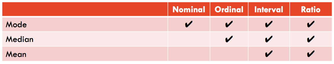
Measures of Central Tendency
Mean
Median
- Value in the middle or an ordered list, or average of two in middle.
Mode
- Most Frequent Value
Quantile
- Division of probability distributions based on contiguous intervals with equal probabilities. In short: Dividing observations numbers in a sample list equally.
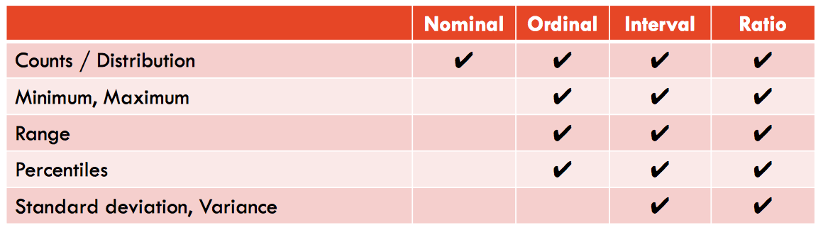
Dispersion
Range
Medium Absolute Deviation (MAD)
- The average of the absolute value of the deviation of each value from the mean
Inter-quartile Range (IQR)
- Three quartiles divide the data in approximately four equally divided parts
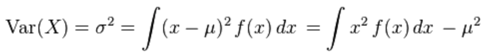
Variance
Definition
- The average of the squared differences from the Mean. Formally, is the expectation of the squared deviation of a random variable from its mean, and it informally measures how far a set of (random) numbers are spread out from their mean.
Types
Continuous
- Discrete
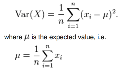
- Discrete
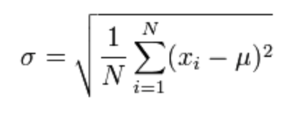
Standard Deviation
sqrt(variance)
z-score/value/factor
- The signed number of standard deviations an observation or datum is above the mean.
Relationship
Covariance
dot(de_mean(x), de_mean(y)) / (n - 1)
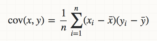
- A measure of how much two random variables change together. http://stats.stackexchange.com/questions/18058/how-would-you-explain-covariance-to-someone-who-understands-only-the-mean
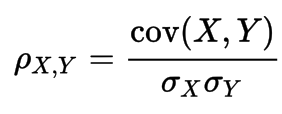
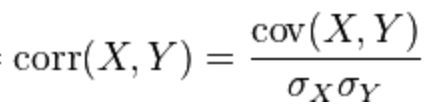
Correlation
Pearson
- Benchmarks linear relationship, most appropriate for measurements taken from an interval scale, is a measure of the linear dependence between two variables
- Benchmarks linear relationship, most appropriate for measurements taken from an interval scale, is a measure of the linear dependence between two variables
Spearman
- Benchmarks monotonic relationship (whether linear or not), Spearman's coefficient is appropriate for both continuous and discrete variables, including ordinal variables.
Kendall
Is a statistic used to measure the ordinal association between two measured quantities.
Contrary to the Spearman correlation, the Kendall correlation is not affected by how far from each other ranks are but only by whether the ranks between observations are equal or not, and is thus only appropriate for discrete variables but not defined for continuous variables.
Summary: Pearson’s r for two normally distributed variables // Spearman’s rho for ratio data, ordinal data, etc (rank-order correlation) // Kendall’s tau for ordinal variables
Co-occurrence
- The results are presented in a matrix format, where the cross tabulation of two fields is a cell value. The cell value represents the percentage of times that the two fields exist in the same events.
Techniques
Null Hypothesis
- Is a general statement or default position that there is no relationship between two measured phenomena, or no association among groups. The null hypothesis is generally assumed to be true until evidence indicates otherwise.
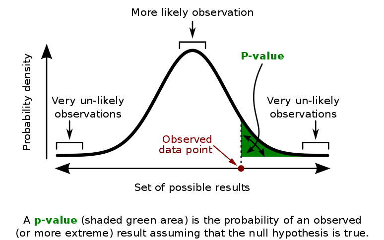
p-value
Five heads in a row Example
This demonstrates that specifying a direction (on a symmetric test statistic) halves the p-value (increases the significance) and can mean the difference between data being considered significant or not.
Suppose a researcher flips a coin five times in a row and assumes a null hypothesis that the coin is fair. The test statistic of "total number of heads" can be one-tailed or two-tailed: a one-tailed test corresponds to seeing if the coin is biased towards heads, but a two-tailed test corresponds to seeing if the coin is biased either way. The researcher flips the coin five times and observes heads each time (HHHHH), yielding a test statistic of 5. In a one-tailed test, this is the upper extreme of all possible outcomes, and yields a p-value of (1/2)5 = 1/32 ≈ 0.03. If the researcher assumed a significance level of 0.05, this result would be deemed significant and the hypothesis that the coin is fair would be rejected. In a two-tailed test, a test statistic of zero heads (TTTTT) is just as extreme and thus the data of HHHHH would yield a p-value of 2×(1/2)5 = 1/16 ≈ 0.06, which is not significant at the 0.05 level.
In this method, as part of experimental design, before performing the experiment, one first chooses a model (the null hypothesis) and a threshold value for p, called the significance level of the test, traditionally 5% or 1% and denoted as α. If the p-value is less than the chosen significance level (α), that suggests that the observed data is sufficiently inconsistent with the null hypothesis that the null hypothesis may be rejected. However, that does not prove that the tested hypothesis is true. For typical analysis, using the standard α = 0.05 cutoff, the null hypothesis is rejected when p < .05 and not rejected when p > .05. The p-value does not, in itself, support reasoning about the probabilities of hypotheses but is only a tool for deciding whether to reject the null hypothesis.
p-hacking
- The process of data mining involves automatically testing huge numbers of hypotheses about a single data set by exhaustively searching for combinations of variables that might show a correlation. Conventional tests of statistical significance are based on the probability that an observation arose by chance, and necessarily accept some risk of mistaken test results, called the significance.
Central Limit Theorem
States that a random variable defined as the average of a large number of independent and identically distributed random variables is itself approximately normally distributed.
- http://blog.vctr.me/posts/central-limit-theorem.html
Experiments and Tests
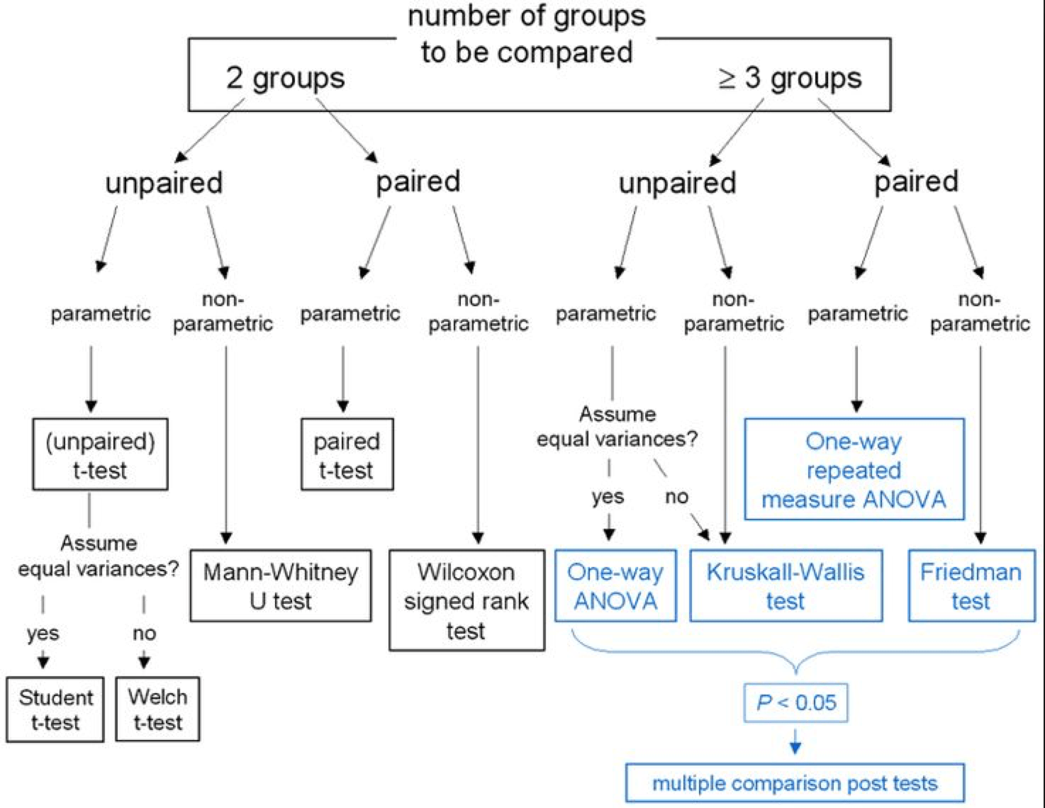
Flow Chart of Commonly Used Stat Tests
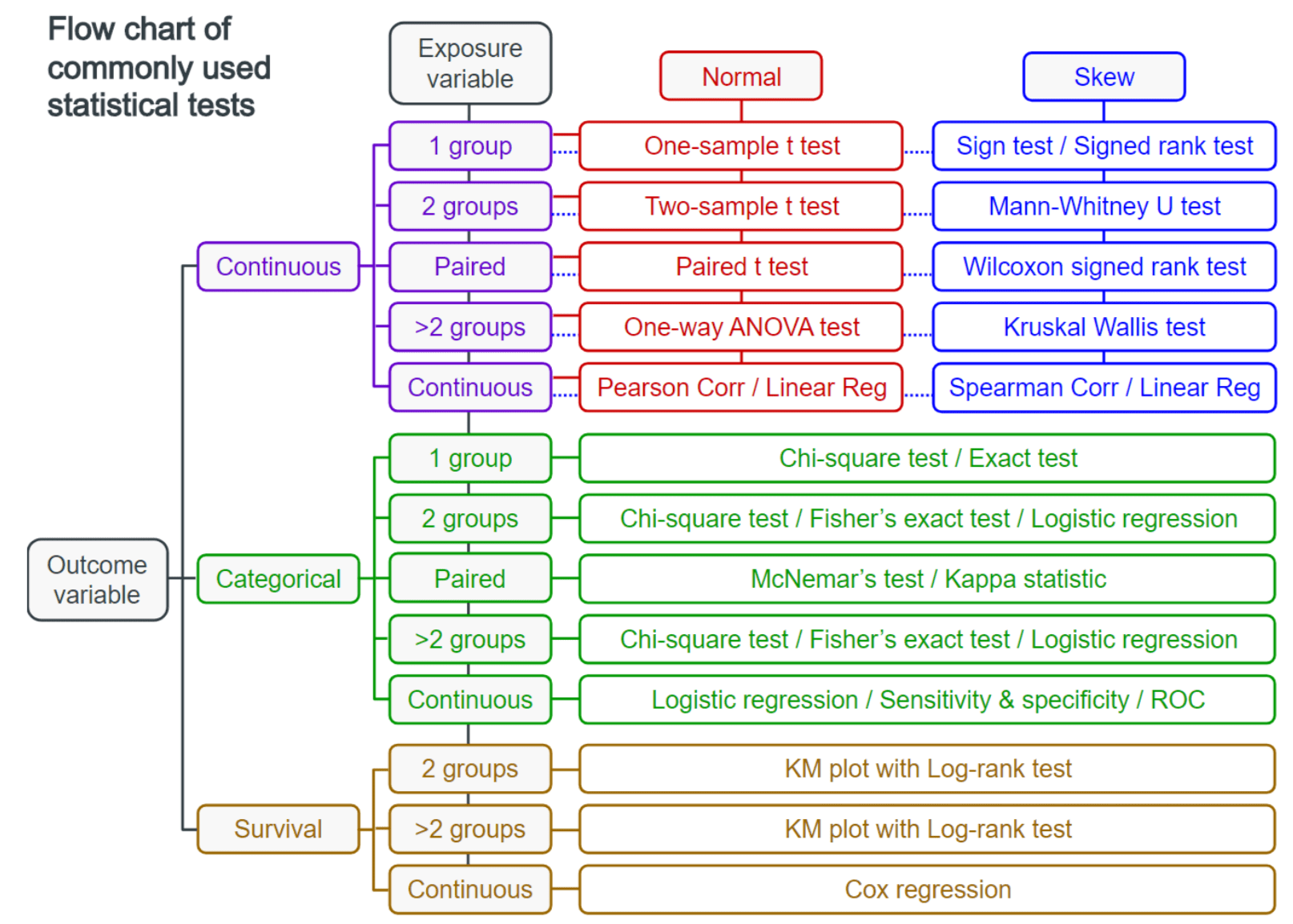
Research Question
Research question (Q):
- Asks whether the independent variable has an effect: “If there is a change in the independent variable, will there also be a change in the dependent variable?”
Null hypothesis (Ho):
- The assumption that there is no effect: “There is no change in the dependent variable when the independent variable changes.”
Types of variables
Dependent variable is the measure of interest
Independent variable is manipulated to observe the effect on dependent variable
Controlled variables are materials, measurements and methods that don’t change
Experiment design
Between subjects: Each subject sees one and only one condition
Within subjects: Subjects see more than one or all conditions
Testing reliability with p-values
Most tests calculate a p-value measuring observation extremity
Compare to significance level threshold α
α is the probability of rejecting H0 given that it is true
Commonly use α of 5% or 1%
Linear Algebra
Matrices
Almost all Machine Learning algorithms use Matrix algebra in one way or another. This is a broad subject, too large to be included here in it’s full length. Here’s a start: https://en.wikipedia.org/wiki/Matrix_(mathematics)
Basic Operations: Addition, Multiplication, Transposition
Transformations
Trace, Rank, Determinante, Inverse
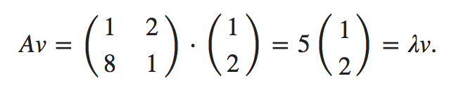
Eigenvectors and Eigenvalues
In linear algebra, an eigenvector or characteristic vector of a linear transformation T from a vector space V over a field F into itself is a non-zero vector that does not change its direction when that linear transformation is applied to it.
- http://setosa.io/ev/eigenvectors-and-eigenvalues/
- http://setosa.io/ev/eigenvectors-and-eigenvalues/
Derivatives Chain Rule
Rule
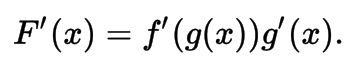
- Leibniz Notation
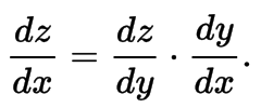
- Leibniz Notation
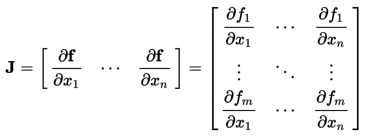
Jacobian Matrix
The matrix of all first-order partial derivatives of a vector-valued function. When the matrix is a square matrix, both the matrix and its determinant are referred to as the Jacobian in literature
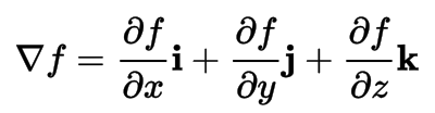
Gradient
The gradient is a multi-variable generalization of the derivative. The gradient is a vector-valued function, as opposed to a derivative, which is scalar-valued.
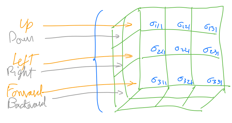
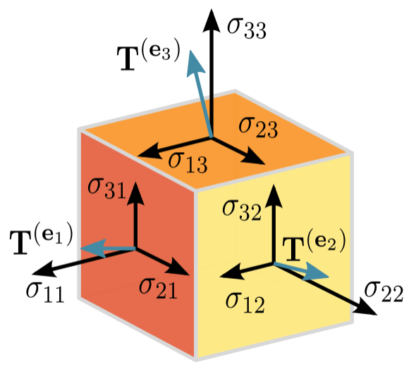
Tensors
For Machine Learning purposes, a Tensor can be described as a Multidimentional Matrix Matrix. Depending on the dimensions, the Tensor can be a Scalar, a Vector, a Matrix, or a Multidimentional Matrix.
When measuring the forces applied to an infinitesimal cube, one can store the force values in a multidimensional matrix.
Curse of Dimensionality
- When the dimensionality increases, the volume of the space increases so fast that the available data become sparse. This sparsity is problematic for any method that requires statistical significance. In order to obtain a statistically sound and reliable result, the amount of data needed to support the result often grows exponentially with the dimensionality.
Machine Learning Data Processing
Feature Selection
Correlation
Features should be uncorrelated with each other and highly correlated to the feature we’re trying to predict.
Covariance
- A measure of how much two random variables change together. Math: dot(de_mean(x), de_mean(y)) / (n - 1)
- A measure of how much two random variables change together. Math: dot(de_mean(x), de_mean(y)) / (n - 1)
Dimensionality Reduction
Principal Component Analysis (PCA)
Principal component analysis (PCA) is a statistical procedure that uses an orthogonal transformation to convert a set of observations of possibly correlated variables into a set of values of linearly uncorrelated variables called principal components. This transformation is defined in such a way that the first principal component has the largest possible variance (that is, accounts for as much of the variability in the data as possible), and each succeeding component in turn has the highest variance possible under the constraint that it is orthogonal to the preceding components.
- Plot the variance per feature and select the features with the largest variance.
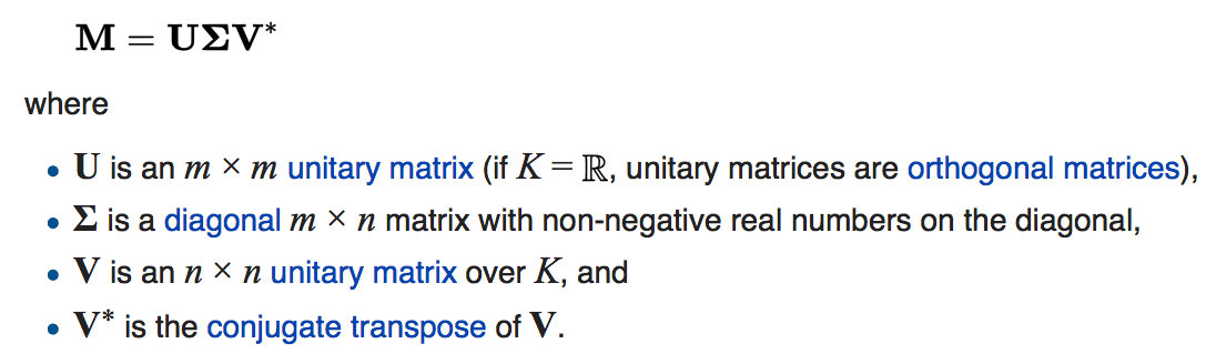
Singular Value Decomposition (SVD)
SVD is a factorization of a real or complex matrix. It is the generalization of the eigendecomposition of a positive semidefinite normal matrix (for example, a symmetric matrix with positive eigenvalues) to any m×n matrix via an extension of the polar decomposition. It has many useful applications in signal processing and statistics.
Importance
Filter Methods
Filter type methods select features based only on general metrics like the correlation with the variable to predict. Filter methods suppress the least interesting variables. The other variables will be part of a classification or a regression model used to classify or to predict data. These methods are particularly effective in computation time and robust to overfitting.
Correlation
Linear Discriminant Analysis
ANOVA: Analysis of Variance
Chi-Square
Wrapper Methods
Wrapper methods evaluate subsets of variables which allows, unlike filter approaches, to detect the possible interactions between variables. The two main disadvantages of these methods are : The increasing overfitting risk when the number of observations is insufficient. AND. The significant computation time when the number of variables is large.
Forward Selection
Backward Elimination
Recursive Feature Ellimination
Genetic Algorithms
Embedded Methods
Embedded methods try to combine the advantages of both previous methods. A learning algorithm takes advantage of its own variable selection process and performs feature selection and classification simultaneously.
Lasso regression performs L1 regularization which adds penalty equivalent to absolute value of the magnitude of coefficients.
Ridge regression performs L2 regularization which adds penalty equivalent to square of the magnitude of coefficients.
Feature Encoding
Machine Learning algorithms perform Linear Algebra on Matrices, which means all features must be numeric. Encoding helps us do this.
Label Encoding
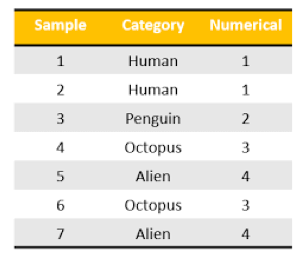
One Hot Encoding
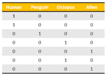
- In One Hot Encoding, make sure the encodings are done in a way that all features are linearly independent.
Feature Normalisation or Scaling
Since the range of values of raw data varies widely, in some machine learning algorithms, objective functions will not work properly without normalization. Another reason why feature scaling is applied is that gradient descent converges much faster with feature scaling than without it.
Methods
Rescaling
The simplest method is rescaling the range of features to scale the range in [0, 1] or [−1, 1].
Standardization
Feature standardization makes the values of each feature in the data have zero-mean (when subtracting the mean in the numerator) and unit-variance.
Scaling to unit length
To scale the components of a feature vector such that the complete vector has length one.
Dataset Construction
Training Dataset
A set of examples used for learning
- To fit the parameters of the classifier in the Multilayer Perceptron, for instance, we would use the training set to find the “optimal” weights when using back-progapation.
Test Dataset
A set of examples used only to assess the performance of a fully-trained classifier
- In the Multilayer Perceptron case, we would use the test to estimate the error rate after we have chosen the final model (MLP size and actual weights) After assessing the final model on the test set, YOU MUST NOT tune the model any further.
Validation Dataset
A set of examples used to tune the parameters of a classifier
- In the Multilayer Perceptron case, we would use the validation set to find the “optimal” number of hidden units or determine a stopping point for the back-propagation algorithm
Cross Validation
- One round of cross-validation involves partitioning a sample of data into complementary subsets, performing the analysis on one subset (called the training set), and validating the analysis on the other subset (called the validation set or testing set). To reduce variability, multiple rounds of cross-validation are performed using different partitions, and the validation results are averaged over the rounds.
Feature Engineering
Decompose
- Converting 2014-09-20T20:45:40Z into categorical attributes like hour_of_the_day, part_of_day, etc.
Discretization
Continuous Features
- Typically data is discretized into partitions of K equal lengths/width (equal intervals) or K% of the total data (equal frequencies).
Categorical Features
- Values for categorical features may be combined, particularly when there’s few samples for some categories.
Reframe Numerical Quantities
- Changing from grams to kg, and losing detail might be both wanted and efficient for calculation
Crossing
- Creating new features as a combination of existing features. Could be multiplying numerical features, or combining categorical variables. This is a great way to add domain expertise knowledge to the dataset.
Feature Imputation
Hot-Deck
- The technique then finds the first missing value and uses the cell value immediately prior to the data that are missing to impute the missing value.
Cold-Deck
- Selects donors from another dataset to complete missing data.
Mean-substitution
- Another imputation technique involves replacing any missing value with the mean of that variable for all other cases, which has the benefit of not changing the sample mean for that variable.
Regression
- A regression model is estimated to predict observed values of a variable based on other variables, and that model is then used to impute values in cases where that variable is missing
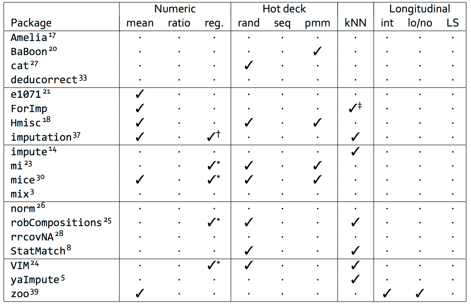
Some Libraries...
Feature Cleaning
Missing values
- One may choose to either omit elements from a dataset that contain missing values or to impute a value
Special values
- Numeric variables are endowed with several formalized special values including ±Inf, NA and NaN. Calculations involving special values often result in special values, and need to be handled/cleaned
Outliers
- They should be detected, but not necessarily removed. Their inclusion in the analysis is a statistical decision.
Obvious inconsistencies
- A person's age cannot be negative, a man cannot be pregnant and an under-aged person cannot possess a drivers license.
Data Exploration
Variable Identification
- Identify Predictor (Input) and Target (output) variables. Next, identify the data type and category of the variables.
Univariate Analysis
Continuous Features
- Mean, Median, Mode, Min, Max, Range, Quartile, IQR, Variance, Standard Deviation, Skewness, Histogram, Box Plot
Categorical Features
- Frequency, Histogram
Bi-variate Analysis
Finds out the relationship between two variables.
Scatter Plot
Correlation Plot - Heatmap
Two-way table
- We can start analyzing the relationship by creating a two-way table of count and count%.
Stacked Column Chart
Chi-Square Test
- This test is used to derive the statistical significance of relationship between the variables.
Z-Test/ T-Test
ANOVA
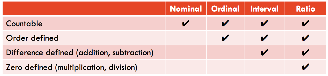
Data Types
Nominal - is for mutual exclusive, but not ordered, categories.
Ordinal - is one where the order matters but not the difference between values.
Ratio - has all the properties of an interval variable, and also has a clear definition of 0.0.
Interval - is a measurement where the difference between two values is meaningful.
Machine Learning Models
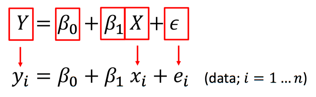
Regression
Linear Regression
Generalised Linear Models (GLMs)
Is a flexible generalization of ordinary linear regression that allows for response variables that have error distribution models other than a normal distribution. The GLM generalizes linear regression by allowing the linear model to be related to the response variable via a link function and by allowing the magnitude of the variance of each measurement to be a function of its predicted value.
Link Function
Identity
Inverse
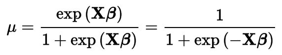
Logit
Cost Function is found via Maximum Likelihood Estimation
Locally Estimated Scatterplot Smoothing (LOESS)
Ridge Regression
Least Absolute Shrinkage and Selection Operator (LASSO)
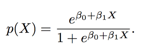
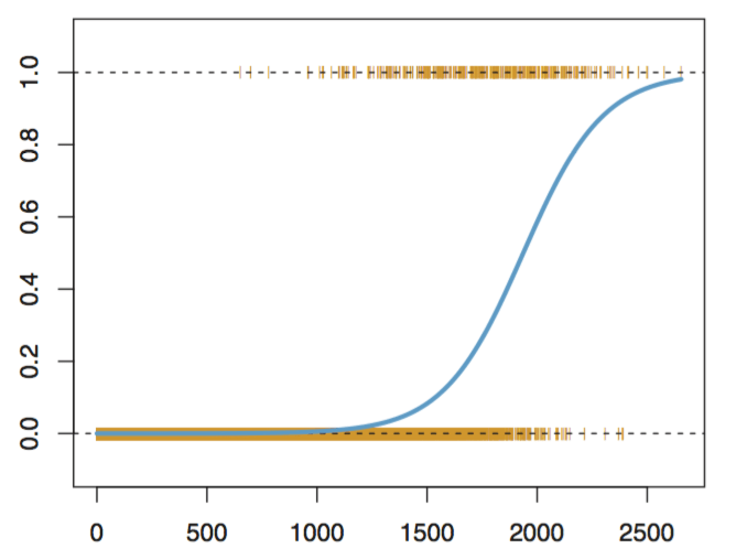
Logistic Regression
Logistic Function
Bayesian
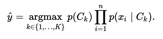
Naive Bayes
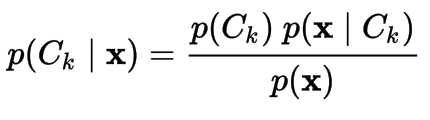
- Naive Bayes Classifier. We neglect the denominator as we calculate for every class and pick the max of the numerator
Multinomial Naive Bayes
Bayesian Belief Network (BBN)
Dimensionality Reduction
Principal Component Analysis (PCA)
Partial Least Squares Regression (PLSR)
Principal Component Regression (PCR)
Partial Least Squares Discriminant Analysis
Quadratic Discriminant Analysis (QDA)
Linear Discriminant Analysis (LDA)
Instance Based
k-nearest Neighbour (kNN)
Learning Vector Quantization (LVQ)
Self-Organising Map (SOM)
Locally Weighted Learning (LWL)
Decision Tree
Random Forest
Classification and Regression Tree (CART)
Gradient Boosting Machines (GBM)
Conditional Decision Trees
Gradient Boosted Regression Trees (GBRT)
Clustering
Algorithms
Hierarchical Clustering
Linkage
complete
single
average
centroid
Dissimilarity Measure
Euclidean
- Euclidean distance or Euclidean metric is the "ordinary" straight-line distance between two points in Euclidean space.
Manhattan
- The distance between two points measured along axes at right angles.
k-Means
- How many clusters do we select?
k-Medians
Fuzzy C-Means
Self-Organising Maps (SOM)
Expectation Maximization
DBSCAN
Validation
Data Structure Metrics
Dunn Index
Connectivity
Silhouette Width
Stability Metrics
Non-overlap APN
Average Distance AD
Figure of Merit FOM
Average Distance Between Means ADM
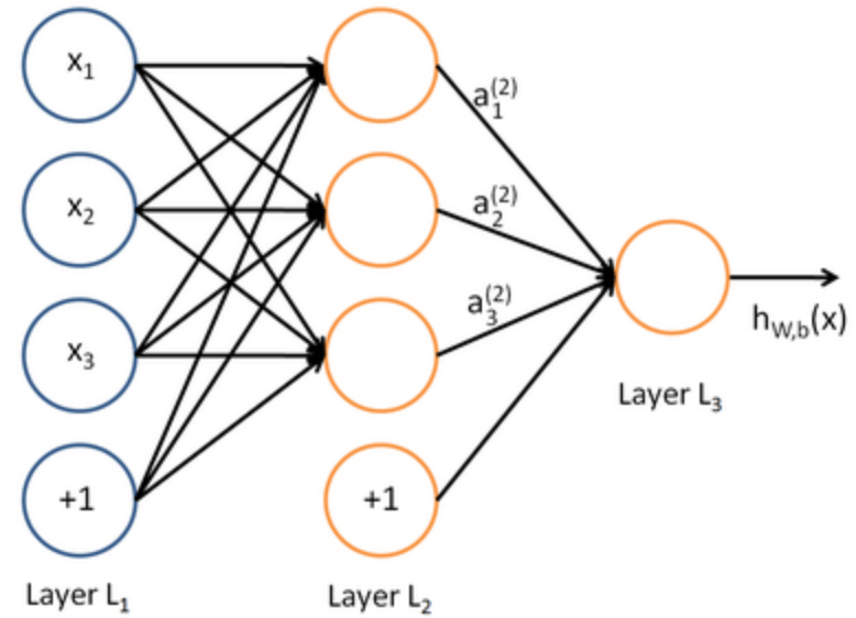
Neural Networks
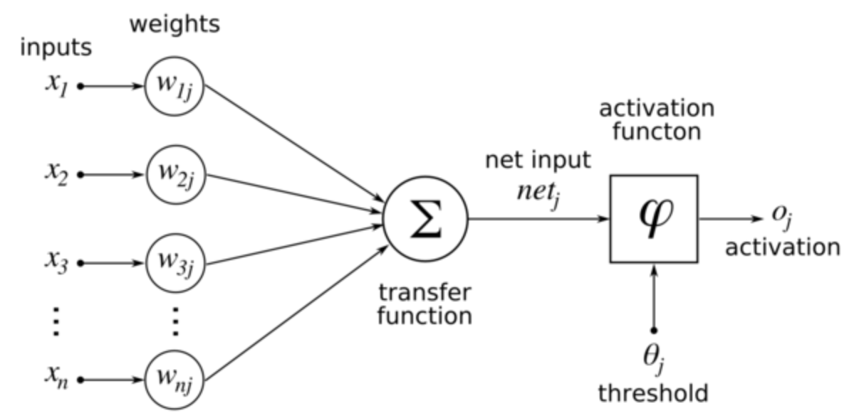
Unit (Neurons)
A unit often refers to the activation function in a layer by which the inputs are transformed via a nonlinear activation function (for example by the logistic sigmoid function). Usually, a unit has several incoming connections and several outgoing connections.
Input Layer
- Comprised of multiple Real-Valued inputs. Each input must be linearly independent from each other.
Hidden Layers
Layers other than the input and output layers. A layer is the highest-level building block in deep learning. A layer is a container that usually receives weighted input, transforms it with a set of mostly non-linear functions and then passes these values as output to the next layer.
Batch Normalization
Using mini-batches of examples, as opposed to one example at a time, is helpful in several ways. First, the gradient of the loss over a mini-batch is an estimate of the gradient over the training set, whose quality improves as the batch size increases. Second, computation over a batch can be much more efficient than m computations for individual examples, due to the parallelism afforded by the modern computing platforms.
- With SGD, the training proceeds in steps, and at each step we consider a mini- batch x1...m of size m. The mini-batch is used to approx- imate the gradient of the loss function with respect to the parameters.
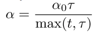
Learning Rate
Neural networks are often trained by gradient descent on the weights. This means at each iteration we use backpropagation to calculate the derivative of the loss function with respect to each weight and subtract it from that weight.
- However, if you actually try that, the weights will change far too much each iteration, which will make them “overcorrect” and the loss will actually increase/diverge. So in practice, people usually multiply each derivative by a small value called the “learning rate” before they subtract it from its corresponding weight.
Tricks
Simplest recipe: keep it fixed and use the same for all parameters.
Better results by allowing learning rates to decrease Options:
Reduce by 0.5 when validation error stops improving
Reduction by O(1/t) because of theoretical convergence guarantees, with hyper-parameters ε0 and τ and t is iteration numbers.
Better yet: No hand-set learning of rates by using AdaGrad
Weight Initialization
All Zero Initialization
In the ideal situation, with proper data normalization it is reasonable to assume that approximately half of the weights will be positive and half of them will be negative. A reasonable-sounding idea then might be to set all the initial weights to zero, which you expect to be the “best guess” in expectation.
- But, this turns out to be a mistake, because if every neuron in the network computes the same output, then they will also all compute the same gradients during back-propagation and undergo the exact same parameter updates. In other words, there is no source of asymmetry between neurons if their weights are initialized to be the same.
Initialization with Small Random Numbers
Thus, you still want the weights to be very close to zero, but not identically zero. In this way, you can random these neurons to small numbers which are very close to zero, and it is treated as symmetry breaking. The idea is that the neurons are all random and unique in the beginning, so they will compute distinct updates and integrate themselves as diverse parts of the full network.
- The implementation for weights might simply drawing values from a normal distribution with zero mean, and unit standard deviation. It is also possible to use small numbers drawn from a uniform distribution, but this seems to have relatively little impact on the final performance in practice.
Calibrating the Variances
One problem with the above suggestion is that the distribution of the outputs from a randomly initialized neuron has a variance that grows with the number of inputs. It turns out that you can normalize the variance of each neuron's output to 1 by scaling its weight vector by the square root of its fan-in (i.e., its number of inputs)
- This ensures that all neurons in the network initially have approximately the same output distribution and empirically improves the rate of convergence. The detailed derivations can be found from Page. 18 to 23 of the slides. Please note that, in the derivations, it does not consider the influence of ReLU neurons.
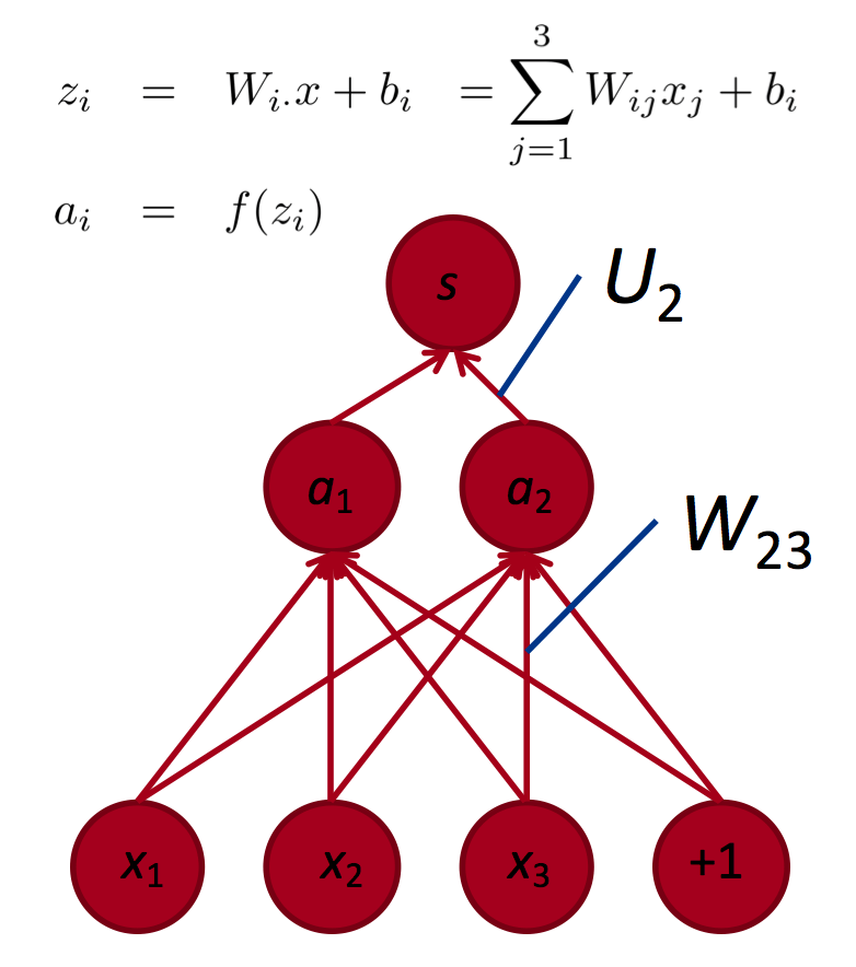
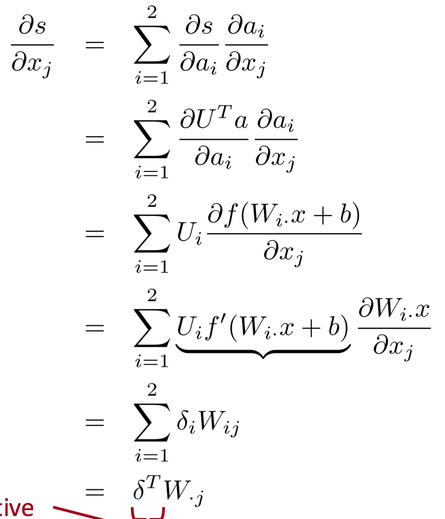
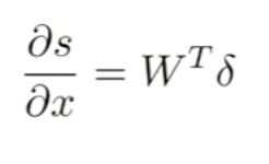
Backpropagation
Is a method used in artificial neural networks to calculate the error contribution of each neuron after a batch of data. It calculates the gradient of the loss function. It is commonly used in the gradient descent optimization algorithm. It is also called backward propagation of errors, because the error is calculated at the output and distributed back through the network layers.
Neural Network taking 4 dimension vector representation of words.
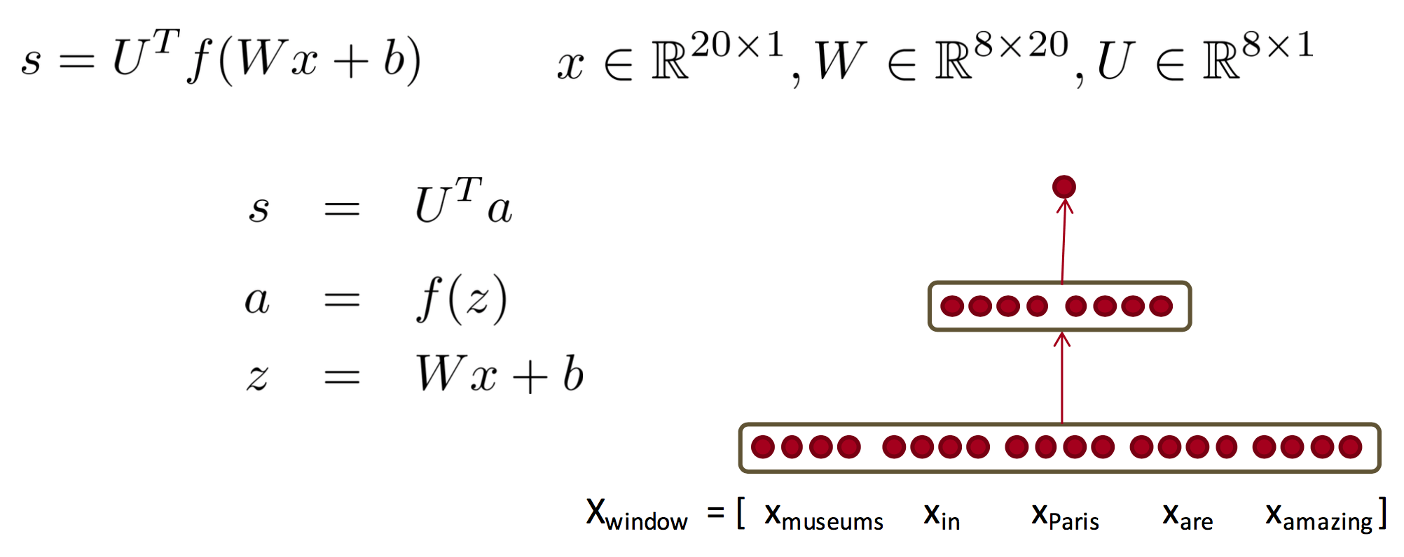
In this method, we reuse partial derivatives computed for higher layers in lower layers, for efficiency.
Activation Functions
Defines the output of that node given an input or set of inputs.
Types
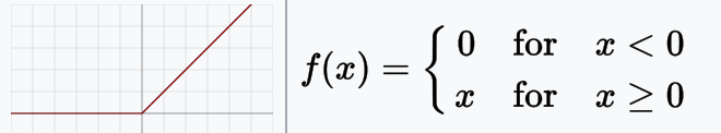
ReLU
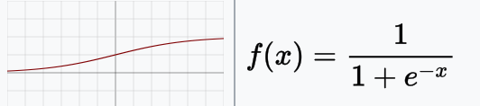
Sigmoid / Logistic
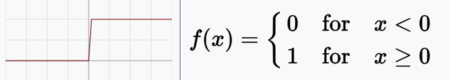
Binary
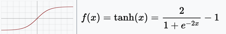
Tanh
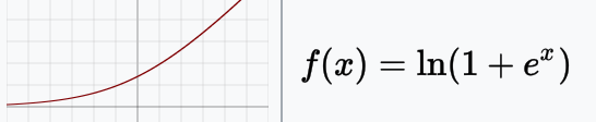
Softplus
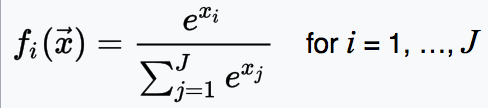
Softmax
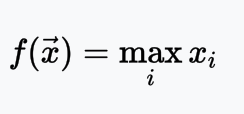
Maxout
Leaky ReLU, PReLU, RReLU, ELU, SELU, and others.